■ numpy.matrix
numpy matrix は dot(..) の代わりに * 演算子を使えるようにしてみただけでに見える。numpy 全体での整合性を保ち広範な利用を追及されているとは思えない。
<== numpy の開発者の大半が matrix ではなく ndarray を使うことしか考えていない。
mt=sc.matrix([[1,2],[3,4]]);(5,6) mt
mt=sc.matrix([[1,2],[3,4]]);[5,6] mt
===============================
[[23 34]]
mt=sc.matrix([[1,2],[3,4]]);mt [5,6]
objects are not aligned at excecuting:mt * [5,6]
mt=sc.matrix([[1,2],[3,4]]);mt mt^-1
sc.matrix([[1,2],[3,4]])^-1
sc.matrix([[1,2],[3,4]])^-1
sc.matrix([[1,2],[3,4]])^2
sc.info(sc)
repr(sc.ndarray([1,2,3, 4,5,6]))
repr(sc.ndarray([1,2,3]))
repr(sc.ndarray([1,2,3]))
repr(sc.arange(10))
sc.arange(10)
mt=sc.matrix([[1,2],[3,4]]);type(sc.fft.fft(mt[0,]))
===============================
~[....] の一番最後に、型変数を書き込むことで、ベクトル行列の要素の型を明示的に指定できます
正方行列の 0 べき乗は無条件に単位行列にしています。たとえ、0 行列の 0 べき乗でも、単位行列にします。0^0 は数学では不定であることは分かっていますが、Python では 0^0 == 1 です。これを踏襲しました。不定なのを単位行列にしても誤りで花からです。また こちらのほうが krzs(8,8)^0 などと簡単に単位行列を定義できて便利だからです。
符号を反転させるために、マイナスを付けるのが嫌ですが、それなりに使えるでしょう
scipy/numpy にも三次元の外積を求める関数 cross があるます。これらのモジュール名には sc の名前をすでにわりふってあります。下のように外せきを計算します。
vpython にも三次元の外積を求める関数 cross があるます。vpython モジュールには vs の名前を割符って有ります
ただし、計算結果は vpython の array になります。三次元専用なので、二次のベクトルを与えても、三次元の外積を計算します。
Wedge 積を `Λ(...) の関数名で customize.py に定義してあります。数学に詳しい方には、Wedge 積関数が、外積計算の方法として一番整合性がとれるでしょう。二次元、三次元、四次元, ... 任意の次元で外積を計算できのるですから。
ただし`Λ(..) による外積計算の結果は反対称行列として出力されるので、数学に詳しくない方は面食らうかも知れませんね。
-->
~[...] による行列生成操作は、既存の python 操作と組み合わせて便利に使えます。
ClTensor が numpy array と大きく異なる点の一つが ^ operator 拡張をしている点です。
ClTensor と tuple, list,dict との演算であっても、tuple, list, dict を行列やベクトルに変換して加減乗除算を行います
sc.ndarray は十分すぎる method を備えています。そして sc.ndarray を継承している ClTensor は、ここれらの method を使えます。
幸いなことに、ClTensor instance に、上のメソッドを適用して帰ってくる行列は ClTensor になっています。
sc.sin は numpy で実装されており、ClTensor 何ぞは知らないにも拘わらず、sc.sin(`σx) は戻り値行列を `σx の型 ClTensor 行列にしてくれる。
scipy 全ての関数が unversal function とは限らない。
sin+cos も universal function です。ClAF は universal function について意識せずにコーディングしてあるのに。
Python の大の機能は直行性を持ちます。整数演算・リスト演算などから類推される機能は行列・ベクトル演算でも満たされるように実装されるべきです。
部分行列についても += 演算ができます。
Bool 体、など、一般体の行列を独立に実装する必要があります。ClFldTns として ClTensor, sc.array とは独立して実装してあります。
scipy.py の行列には object タイプの行列があります。
ar=sc.array([oc.Pl(oc.RS(2), 1), oc.Pl(oc.RS(4), 1)], dtype=object);ar+ar
===============================
[0 0]
ar=sc.array([oc.Pl(oc.RS(2), 1), oc.Pl(oc.RS(4), 1)], dtype=object);ar oc.RS(5)
===============================
[0x0ax+0x05 0x14x+0x05]
ベクトル演算は可能です。
ar=sc.array([oc.Pl(oc.RS(2), 1), oc.Pl(oc.RS(4), 1)], dtype=object);sc.dot(ar, ar)
下と同じです。
oc.Pl(oc.RS(2),1)^2+ oc.Pl(oc.RS(4), 1)^2
ar=~[`1,`0,`1,`1]
===============================
[1 0 1 1]
---- ClFldTns:
できるだけ多くの対象の norm を計算しようと努力しています。数値をもつコンテナ:リスト・タプル、辞書、ベクトル、行列、ClTensor の他に数値を返すイタレータも対象にします。
戻り値は double 精度の浮動小数点値になります。
norm(..) と normSq(..) は殆ど同じです。
戻り値が norm(..) の自乗値になっていることと、integer 要素のコンテナについては integer 値になることが異なります。
「sy();import sy.lib.lapack」の書き方はできません。__init__.py の構造のためです。
sympy モジュールの機能を使うことで、python/python sf でもシンボル式を扱えます。
でも x,y,z シンボルが定義されるわけではありません。
`x `y `z `t 変数については 二階微分 ∂2x,∂2y,∂2z,∂2t も customize.py に定義してあります。
zeta 関数の下のような位相回転を含む 3D 関数を計算できるだけでも、十分に凄まじいと思ってください。scipy で計算できる zeta 関数は実数に限られますから。Viva sympy!
これぐらいになると netbook:N280 では数分掛かります。メール・チェックの間の時間に計算させました。
sympy のシンボルを使って行列操作を行うことも可能です。
でも、シンボル式の演算結果が簡約されているわけではありません。
上のような逆行列式が計算されたとき
sympy シンボル式の計算結果が数値になったとしても、それは sympy の数値です。scipy などの関数引数には使えません。なので python の float/complex 型の変数にする必要があります。
tr();`Rat(1,3)
===============================
1/3
tr();`Rat(1,3) * 2.0
===============================
0.666666666666667
tr();float(`Rat(1,3))
tr();float(`Rat(1,3))*2.0
tr();type((`Rat(1,3))*2.0)
===============================
また sympy 関数式に引数を与えて数値を出させるとき .subs(...) と書かねばなりません。これは書くのも読むのも面倒です。
`x,`y,`z,`t, `p,`q, `n_ のシンボルで記述される sympy 式に限定されますが、これらの式は Float(式, 引数値) または Complex(式, 引数値) で float/complex 値を返すようにしたくなります。その機能を Float/Complex 関数に実装しました。F:\my\vc7\mtCm
関数側で sympy.core.numbers.Real/Complex を受け付けるようにする考え方はとれません。sin,cos などの基本数値関数に限れば、そのようにできます。でも ClRtnl など python で定義される関数の大部分は sympy.core.numbers.Real/Complex については考慮していない関数だからです。
もし無理やりに sin,cos.. などの基本数値関数を「sympy.core.numbers.Real/Complex を受け付ける関数に改造してやる」とすると、関数の動作に二種類のものができてしまうことになります。これ耐えられないことだと考えます。
なお ts() は customize.py に実装しています。暇なときにでも、こちらのソースを読んでもらえたらと思います。
特に専用のアイコンで書かれたボタンを用意しています。マウスで終了させたければ、ウィンドウの右上にある × をクリックしてください。
Windows 標準で備わっているキーボーデでの終了のやりかた:「ctrl+space→ C」 のほうが素早く衆力できると思います。
vsGraph は 二次元グラフ表示関数:plotGr(..), 二次元/三次元の軌跡表示関数:plotTrajectory(..)、三次元グラフ表示関数:plot3dGr(..),タイムチャート表示関数:plotTmCh(..) などのデータ表示のための関数を実装してあります。
これらは Python sf のワン・ライナーでも扱いやすいように、最小の手間で最大の情報を表示させるように実装されています。最小の手間、論文などの赤の他人に読ませるための凡例など多くの情報をちりばめたグラフを作成するためには、pylab などのグラフ表示パッケージを使うべきです。
help(vsGraph)
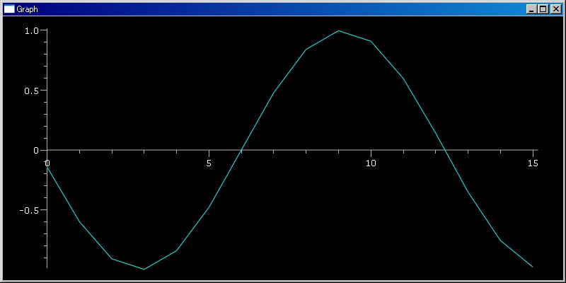
最も多用されるグラフ表示は一変数関数の二次元表示 plotGr(..) でしょう。
でも、plotGr(..) 関数には多くの機能詰め込んでいます。上に書いてある説明では不十分です。Python のソースが読めるならば plotGr(..) を詳細に理解する一番の方法は Python のシースを読むことです。
Python のソースを追うような真似をせずにグラフ表示をさせたいならば「plotGr(関数, 開始位置:デフォルト0、終了位置:デフォルト1)」と「plotGr(シーケンス・データ)」の二つのグラフ表示方法を使い分けることにしておけば良いでしょう。
グラフ表示区間の開始位置、終了位置の数値引数を追加してやれば、その区間のグラフ表示をします。
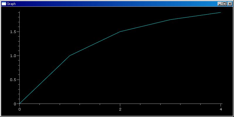
plotGr(..) にシーケンス・データを与えてやれば、その与えられた点を直線で結んだ折れ線グラフを表示します。50 点以上のデータを与えてやれば、ディスプレー上では折れ線ではなく連続しているように見えるようになります。ただし、このとき横軸はシーケンス・データのインデックス整数値になります。シーケンス・データとしては lit, tuple, sc.ndarray ベクトル, ClTensor ベクトル何れでもグラフを表示します。
IMG
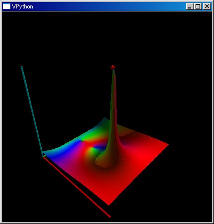
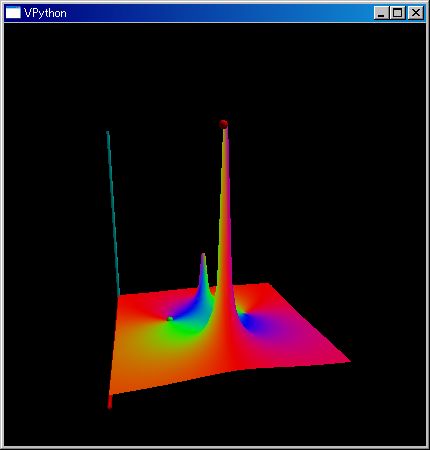
表示領域内で complex 値をとると 3d kkRGB 表示になります。
vsGraph.py ソース・コードも公開されています。それらを見てもらえば、ユーザーが望むグラフ表示関数を作ることも容易であることを分かってもらえると思います。
plotG(..) は、最小の手間で一変数関数のグラフを描くことを目指した関数です。
help('plotGr')
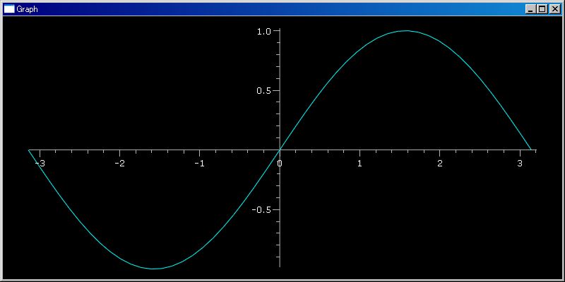
plotGr(sin)
plotGr(sin,-pi,pi)
plotGr(sin,[-pi,pi])
plotGr(sin,klsp(-pi,pi))
plotGr(sin,[-3,-2,-1,0,2 4])
plotGr(sc.sin,[-3,-2,-1,0,2, 4])
plotGr(sin+cos,[-3,-2,-1,0,2 4])
sin+cos([-3,-2,-1,0,2 4])
sc.sin([-3,-2,-1,0,2 4])
引数に関数と lower bound, upper bound の値を与えることでグラフを表示できます
plotGr(..) は、一変数のグラフ表示を最小の手間で行わせる関数です。
引数にリスト、タプル、scipy ベクトル、ClTensor ベクトルを与えることで、折れ線グラフを表示できます。長さを 32 以上にすれば曲線と変わらなくなってきます。
引数に関数と [lower bound, upper bound] を分割したシーケンスまたはイタレーターを与えることでグラフを表示できます
グラフの色指定と重ね合わせ表示が可能です。
plotGr(fn, .....) で fn が複素数値をとる関数のときは実数部分のみを表示します。
plotGr(..) は重ねがきはできますが、ディジタル信号のタイムチャートのように複数の信号を表示するのに向きません。そこで plotTmCh(..) に 行列データを与えることで、タイムチャート表示を可能にしました。
1,0 のデジタル信号だけに限らず、アナログ信号の複数表示も可能になっています。
plotTrajectory
もっと詳細なグラフ表示を望むユーザーも多いかもしれません。背景表示が黒が気にいらない方もいるでしょう。そのような方は是非、御自分で plotGr(..) のような関数を作ってください。難しく有りません。plotGr(..) などのソースも公開してあります。90 行程度です。後で述べる python sf のカスタマイズ機能により、ユーザーが書いた関数やクラスなどを Python sf で使えるようにできます。
basicFnctns.py に入っている基本数値関数群についての説明です
ClAF/ClAFM は、関数の加減乗と合成を可能にする関数のラッパー・クラスです。ClAF が一変数のみの引数の関数のためのラッパークラスです。ClAFM は多変数引数のラッパー・クラスです。
下のように、ClAF(.) でラップされた一変数関数は絵加減乗算が可能になります。
関数の除算は入れていません。0 div エラーを嫌ったためです。
下の関数 g の戻り値が [2x+y, x+2y] と長さ 2 のシーケンスになっています。これにより f(..) の二個の引数と合成が可能になっています。
基本数値関数と一般関数の加減乗算も可能です。
でも、λ 式のときは括弧で囲んで、式の境界を明示してください。Python 自体が parse エラーを起こします。
このような関数自体で加減乗除べき乗算と関数合成が許される関数は、デフォルトでは Python sf 基本関数だけです。ビルトイン math モジュールの math.sin や特殊関数 scipy.special.erf など、Python で使われている関数自体には加減乗除べき乗算・関数合成に対応する演算子は実装されていません。
でも、一変数関数ならば ClAF(userFnction) でラップするだけで Python sf 基本関数と加減乗除べき乗算・関数合成が可能になります。
上で出てくる関数は全て一変数関数です。`Y,`Z,`T が 1st,2nd,last と引数タプルから値を抜き出す位置が特定されている特殊な恒等関数なのですが、これらも一変数関数です。
この様な一変数関数の加減乗除べき乗算と関数合成で作られる多変数関数の集合は、一般の多変数関数の集合より ずっと小さい集合にすぎません。でも我々が使う多変数関数の殆どが、このような一変数関数の加減乗除べき乗算と関数合成の組み合わせによる多変数関数です。
逆に、一般の多変数関数の加減乗除べき乗算と関数合成を Python で記述しようとしても、その体系は複雑怪奇になりすぎて記述できません。
sf.putPv(..) 関数は行列値など、Python でのインスタンス一般を python の pickle 機能を使って、カレント・ディレクトリに保存しています。残念ながら、pickle ではテキスト・ファイルで保存するのですが、その中身は人間が読むようには作られていません。行列以外のインスタンスもテキストで保存することを想定すれば納得してもらえると思います。
でも Python sf で使う ClTensor のインスタンスならば、人間が読める形式で、カレント・ディレクトリに保存します。
そのテキスト・ファイルは、下のように人間が読めます。
putPv(..) でカレント・ディレクトリに作られたファイル変数は getPv(...) で読み戻せます。Python sf プリプロセッサでは「=:」によっても、読み戻せます。
shftSq(..) はシーケンスデータのシフトした値を返します。シフトされた後には 0 が挿入されます。二番目の引数でシフト回数を指定できます。マイナスのシフト回数は左側にシフトします。
シーケンス・データの型を保ちます
rttSq(..) はシーケンスデータを回転した値を返します。二番目の引数で回転の回数を指定できます。マイナスのシフト回数は左周りの回転をさせます。
シーケンス・データの型を保ちます
invF(関数、定義域初め、定義域終わり) は関数引数の逆関数を返します。定義域の範囲で一価関数でなければなりません。すなわち単調でなければなりません。
scipy.optime の brentq(..) を使って実装しています。
n 個の組み合わせを返すジェネレータです。
辞書式順序で返します。
シーケンス引数に対する順列組み合わせを順次返していくイタレータを生成します。順列の入れ替えに対応する sign:-1 or 1 も返します。
permutate 関数の応用例として、wedge 積を計算する `Λ(..) 関数を見てみましょう。下のように、広い範囲の引数をとる wedge 積関数を簡単に記述できます。
こんな具合に計算できます
一変数関数の組から、合成関数を作って返します。cmps の別名を定義してあります。
compose(f,g)(x) は関数の合成:f(g(x))を行います。
cmps の別名も、compose と全く同じものです。
整数値を binary 表記したときの文字列を返します。Python 3000 のバイナリ表記と同じです。
整数値を binary 表記したときの文字列を返します。引数が浮動小数点でも整数にしてしまいます。デフォルトでは 0 が連続する上位ビットは表示しません。二番目の引数に 1 以上のビット・サイズを指定医すると、その 0 ビットが連続する上位ビットも表示するようになります。
4 ビットごとに '_' を挿入することで、ユーザーにビット位置を解りやすくします。
二番目のビット長を指定する引数よりも、一番目の数値によるビット長を優先します。
行列・ベクトルデータの pretty print です。小数点以下の値が 0 ならば浮動小数点値でも、少数点以下を表示しません。複素数で実数成分/純虚数成分のどちらかが 0 のときは、それを表示しません。
行列・ベクトル・データをできるだけ簡単な、手で書くときに近い表示で表現します。特に複素行列の表示に有効です。
invF に「実数を引数とし実数を戻り値とする一変数の関数:f」を与えると、f の逆関数を返します。デフォルトでは [-1,1] の定義域から f(x) == 値 を満たす x を scipy.optimize.brentq を使って探します。
brentq を使うため「invF(f, rangeLeft=-1,rangeRight=1)(a)」を計算するためには「 f(rangeLeft) < a < f(rangeright)」をユーザーは保証せねばならない。
kNumeric は微分、積分、偏微分、偏微分方程式の solver を Python sf ワンライナーでも扱えるようにします。
関数 f(x) を区間 [a,b] で積分します。
scipy の integrate.quad を殆どそのまま使っています。これは適応的自動積分のアルゴリズムで積分しており、被積分関数の変動がが激しい箇所では積分点を細かく取り、穏やかな箇所では粗く取る積分アルゴリズムです。
積分範囲を ∞:sf.inf にまで広げられます。
ただし、sc.inf を含む積分範囲は、大小関係を逆転させないで下さい。エラーになります。
scipy.integral の quad 積分は、その計算精度と組で結果を返すので、電卓的な用途では面倒になることが多いので qdrt を設けました。計算精度が必要なときは、quad を使ってください。
quadAn(..) は複素平面状での線積分を行います。。引数に解析関数と その積分経路のシーケンスを与えることで、積分経路に沿った積分値を計算します。
ただし解析関数は多価関数になりうるにも関わらず scipy で実装されている解析関数は、主値のみを返す一価関数であることに注意してください。
注意1!! quadC による複素数平面での計算には、∫計算での誤差が付きまといやすい。特に複素平面での exp で発散していくときに数値積分計算に、大きな誤差が付きまとう。複素平面での値分布をイメージできていないときは、quadC ではなく quadAn を使うべき。quadAn は、計算結果の誤差推定値を出してくれるから。
注意2!! si.quad には、被積分変数以外のパラメータのタプルをを args キーワード引数を使って渡せます。でも quadAn(..) では、まだ そこまでの実装をしていません。 quadC は引き渡せるようにしました。
quadGN(..) は、N 次元空間での N 次元ベクトル分布の線積分を計算します。
下では三次元空間での電場分布に対して線積分を計算させています。
quadGN(..) は、N 次元空間での N 次元ベクトル分布の線積分を、Gauss 積分法を使って計算します。quadN(..) は scipy.quad(..) を使って計算させていることだけが異なっています。
下では三次元空間での電場分布にたいし線積分を計算させています。
scipy.integrate.odein(..) を複素数値関数にも適用できるように拡張しました。
一次元調和振動子
二次元調和振動子を複素領域での Hamiltonian で計算させる。一次元のときとはことなり、運動量成分:純虚数成分は表示しない。
常微分方程式の右辺式の呼び出される時刻は scipy 側で定める。引数に与える時刻:sf.arSqnc(0,N,5.0/N) に右辺式を呼び出すわけではない
nearlyEq(..) 関数は浮動小数点値を変数、シーケンス・データ、行列、ベクタが相対的に 6 桁まで一致するとき True を返します。
浮動小数点値の数値計算には誤差がつき物です。理論的・理想的には等式が成り立っても、数値計算では非常に近い値になるだけで、等式が成り立たないことが頻繁に発生します。ですから 浮動小数点値は等しいことを == 演算して比較しても、理論的には True であっても、浮動小数点値が僅かに異なるため False になることも頻繁に発生します。このとき nearlyEq(..) を使うことで、浮動小数点変数、シーケンス・データ、行列、ベクタが殆ど同じ値であることを調べられます。
漸化式を繰り返し適用し、任意の偏微分方程式を数値的に解く solveLaplacian(..)/solvePDE(.) 関数/itrSlvPDE(..) イタレータ関数を用意しました。その使い方、応用例を以下に示します。
この三つの関数は全て境界条件行列を与えて、偏微分方程式に対応する漸化式を繰り返し適用して数値解を求めます。ここでの肝は、境界条件行列と漸化式です。
偏微分方程式の漸化式は教科書に多く説明されててます。でも、ここの境界条件行列は Python sf オリジナルなものです。まず これを説明します。
sf.py モジュールを使って偏微分方程式を解くためには境界条件を表す辞書行列(以下では境界条件行列と呼びます)を作らねばなりません。それを solveLaplacian(..), solvePDE(..), itrSlvPDE(..) python 関数 の dctBoundary 引数に与えることで漸化式の繰り返し処理が行われます。
境界条件行列は sf.py モジュールが扱える偏微分方程式の定義域も定めます。その定義域は n 次元直方体領域に限られます。n 次元直方体領域を同じサイズの小さな n 次元直方体で分割し、そのメッシュ点上の値を数値解として計算します。円形領域は扱えません。二変数のときは長方形の領域のメッシュ上の数値解を求めることになります。
境界条件行列:ここでは より具体的に solvLapalacian(..), solvePDE(..), itrSlvPDE(..) の dctBoundary 行列引数の行列サイズは、メッシュ点上の数値解として求めようとしている行列と同じサイズの辞書行列となります。(逆に言えば dctBoundary の行列 column/row サイズより、偏微分方程式の数値解を保存する行列 column/row などのサイズを sf.py 側で定めます。) dctBoundary 行列は各メッシュ点の性質を表現する辞書行列だともいえます。dctBoundary 辞書行列の各要素には True, False, 文字または境界値のいずれかの値を設定します。
境界条件行列の全ての端面が固定値になっているとは限りません。端面で True になっている箇所がありえます。でも短面では多くの場合漸化式を適用できません。漸化式のインデックスが境界の外側になってしまうものを含むことが多いからです。Python sf では端面で True になっている箇所では、デフォルトで線形外挿補間を行っています。これにより端面での特殊処理を考えない単純な漸化式でも、偏微分方程式の数値解もとめられるようにしました。
漸化式を使った偏微分方程式の数値解は、発散との戦いになります。適切な漸化式を適切な刻み幅で扱ってやらないと簡単に発散します。
でも「(∂x)^2 φ + ∂y)^2 φ==0」のような Laplacian 偏微分方程式は、非常に発散しにくい性質があります。ですので漸化式を Python sf 側で用意したもの Laplacian 偏微分専用の solveLaplacian(..) 関数を用意しました。solveLaplacian(..) では漸化式を用意することなく、境界条件行列を与えるだけで、解を求められます。
本来は「(∂x)^2 φ + ∂y)^2 φ==0」の解は無限遠点で 0 になる境界条件で解くことが多いでしょう。でも、上では内側の境界条件しか与えていません。ですから Python sf は端面がフリーだと判断し線形補完を行って数値解を求めています。その結果、端面より一つ内側が 0 になる数値解になってしまいました。
このよな近似解でも厳密解の基本的性質を反映しています。中央に与えた 3 x 3 の 1 となる境界条件は、この近似解で満たしています。無限遠で 0 になろうとする傾向も、近似解から伺えます。あたかも平面ゴム膜を中央の 3 x 3 の四角だけ境界値 1 に伸ばしたよう全体の解の形が、この近似解からも十分に読みとれます。
有限要素方を使うならば、外側ほど粗くなるメッシュを使って、無限遠点で 0 になる条件により近い解を求めます。でも、そのような解は上の二行で計算させることは無理です。
誤差は大きくても手軽に計算できる solveLaplacian(..) も計算ツールの一つにできます。用途に応じて使ってください。
Laplacian 偏微分方程式以外は、ユーザー側で安定な漸化式を用意せねばなりません。そのために solvePDE(..) を用意しました。多くの場合は try and error で slovePDE(..) を何度か計算させることになると思います。
ここでは「(∂x)^2 φ - ∂y)^2 φ==0」の波動方程式を例に solvePDE(..) の使い方を見てみましょう。端点固定された紐の振動の時間変化を解くことになります。紐の両端:[0,1]を 0 に固定し、時刻 0 での紐の形を sin(2pi x) の形とする初期条件を mtBndry[:,0] に sin(2 pi x) の値を入れることで指定します。紐の速度成分が 0 であることを mtBndry[:,0] に sin(と mtBndry[:,1] が mtBndry[:,1] と同じことで表現します。
上で初期条件を保持している境界条件行列:mtBndry に「def f(mt,(j,k)): mt[j,k]=2mt[j,k-1]-mt[j,k-2]+(timeWidth*M/N)^2 (mt[j+1,k-1]+mt[j-1,k-1]-2mt[j,k-1])」の漸化式を何回も適用して収束させた行列戻り値が、波動方程式の解となります。定存波としての紐の振動の様子が、この数値解から見てとれます。
下のように強制振動を与えることもできます。紐の一方の端を sin(t) で一周期だけ振ってやり、残りの時間は 0 で固定する境界条件は、下の境界条件行列で表せます。
上のように長いワンライナーを使うべきではないという考え方もあると思います。でも全画面表示にすれば、このワンライナーは一行が画面の中に納まっています。同時に、このワンライナーは「(∂x)^2 φ - (∂t)^2φ = 0」の方程式解を計算させるのに共通して使えます。一種の Python モジュールのように使えます。この意味で、このような Python sf ワンライナーも使う価値があります。
itrSlvPDE(..) は漸化式の計算をループで行うために用意しました。それ以外は solvePDE(..) と同じです。上の solvePDE(..) で使った漸化式処理は、itrSlvPDE(..) では下のようになります。上と同じ結果になります。
dct2(sq) は、離散 Cos_II 変換を行います。
多項式nemerator/多項式denominator.plotBode(..) とやると 多項式denominator.plotBode(..) を表示してしまいます。「.」が「/」より優先するからです。(多項式nemerator/多項式denominator).plotBode(..) と括弧が必要です
Bode 線図 plotBode(..) は gain 軸は db ではなく、絶対値の桁数を表示しています。
python には itertools という標準モジュールがあります。遅延評価されるジェネレータを使った、繰り返し記述に便利な関数:ジェネレータのライブラリです。
でも itertools は数列・級数を扱うのには適していません。[..] によるインデックス機能がないからです。逆に itertools にインデックス機能を追加してやれば無限列を扱えるようになります。
mkSrs は make infinite series の省略形です。
gain 1 になる ω を求める
サンプリング間隔にご注意ください。デフォルトで 256 point step 応答です。サンプリングが荒すぎると、サンプリングに伴う折り返しが発生します。
kmayavi.py は、mayavi mlab の、素晴らしい表示機能を one liner で扱えるようにするために設けました。mlab は表示機能を使うためには、多くの場合手間がかかりすぎます。そのままでは、とても one liner で使えません。
なお、mayavi, mlab のバージョンごとの仕様変化が 未だ激しく発生しています。2010.05.31 現在、下のバージョンでテストしています
mayavi の quiver3d(..) 関数はベクトル分布を表示する関数です。便利な関数なのですが、mgrid, ogrid で記述することを前提としており、記述性、ドキュメント性が犠牲になります。mgrid, ogrid を使ったほうが、処理速度が早くなることは分かるのですが、Python sf ワンライナーでは使うことは困難です。そこで kqvr3d(..) を作りました。
vpython で作り直したほうが、より早いものにできそうです。矢印の色と長さを設定するルーチンを作るのが大変です。
kqvr3d(..) に位置分布値とベクトル分布値の両方を与えると、X,y,Z 軸の位置の値は位置を示すものになります。
ワンライナーでは if the else 構文を書かずに済ませるへきですが、で if the else を書きたいときも、あります。そのときは Python 2.5 からサポートされるようになった三項演算子を使えます。
ワンライナーの closure 関数の内部では、外部のループ変数を参照できません。リスト内包表記でも、同じ問題があります。
通常のファイルに書かれる Python コード では、ループ変数を closure 関数内部から参照可能です。
scipy の poly1d が変な動きをしています。
sc.poly1d だけを特別扱いするコードを足してやれば対策できます。でも元がおかしままにしておいて、正しいコードに無理やりなコードを挿入したくありません。
この他にも scipy の poly1d は変な動きをします。
どうしても多項式行列を使いたいときは oc.Pl をお使いください。
scalarStt に値が設定されるのは、python sf 計算結果が実数・複素数値のときです。
コンピュータでの実数・複素数計算値には誤差がつき物です。理論値どおりにはなりません。kVerifier では、実数型の変数については誤差を許容する比較を行います。デフォルトで 1e-6 以下の誤差ならば __compare は正しいと判断します。
■ ベクトル・行列宣言
ベクトル・行列要素の型指定
~[1,2,3, complex]
===============================
[ 1.+0.j  2.+0.j  3.+0.j]
---- ClTensor ----

~[[1,2,3],[4,5,6],int]
===============================
[[1 2 3]
 [4 5 6]]
---- ClTensor ----
ベクトルの内積
Python sf でのベクトル同士の積は内積の意味になります。ただし複素ベクトルの積はユーザーが明示的に複素共役であることを「.d」属性で指定してやらねばなりません。数学でのように勝手に複素共役に変換して内積をとることはありません。特殊相対論での、このような内積の取り方が多用されるため、こちらを選択しました。
a =~[`i,2,3];b=~[4`i,5,6];a b
===============================
(24+0j)

a =~[`i,2,3];b=~[4`i,5,6];a.d b
===============================
(32+0j)
0 行列の 0 べき乗
0^0
===============================
1

mt=~[[1,2],[3,4]]; mt^0
===============================
[[ 1.  0.]
 [ 0.  1.]]
---- ClTensor ----

mt=~[[0,0],[0,0]]; mt^0
===============================
[[ 1.  0.]
 [ 0.  1.]]
---- ClTensor ----

mt=~[[0j,0],[0,0]]; mt^0
===============================
[[ 1.+0.j  0.+0.j]
 [ 0.+0.j  1.+0.j]]
---- ClTensor ----
外積
下のような Levi Civita テンソル `εL も配布ファイルの中の customize.py ファイルに定義してあります。これを使えば、三次元ベクトルの外積を計算できます。
`εL
===============================
[[[ 0.  0.  0.]
  [ 0.  0.  1.]
  [ 0. -1.  0.]]

 [[ 0.  0. -1.]
  [ 0.  0.  0.]
  [ 1.  0.  0.]]

 [[ 0.  1.  0.]
  [-1.  0.  0.]
  [ 0.  0.  0.]]]
---- ClTensor ----

-~[1,2,3] `εL ~[4,5,6]
===============================
[-3.  6. -3.]
---- ClTensor ----
sc.cross([1,2,3], [4,5,6])
===============================
[-3  6 -3]
vs.cross([1,2,3], [4,5,6])
===============================
<-3, 6, -3>
unpicklable

vs.cross([1,2], [4,5])
===============================
<0, 0, -3>
unpicklable
`Λ([1,2],[4,5])
===============================
[[ 0. -2.]
 [ 2.  0.]]
---- ClTensor ----

`Λ([1,2,3],[4,5,6])
===============================
[[ 0. -3. -6.]
 [ 3.  0. -3.]
 [ 6.  3.  0.]]
---- ClTensor ----

`Λ([1,2,3,4],[4,5,6,7])
===============================
[[ 0. -3. -6. -9.]
 [ 3.  0. -3. -6.]
 [ 6.  3.  0. -3.]
 [ 9.  6.  3.  0.]]
---- ClTensor ----
注意
krry([[1,2]])
===============================
[[ 1. 2.]]
---- ClTensor ----
~[[1,2]]
===============================
[ 1. 2.]
---- ClTensor ----
~[...] 操作
j,k=3,4;~[j*[k*[1]]]
===============================
[[ 1.  1.  1.  1.]
 [ 1.  1.  1.  1.]
 [ 1.  1.  1.  1.]]
---- ClTensor ----
ClTensor 属性による操作
mt=~[[1,2],[3,4]]; mt.m_inv
===============================
[[-2. 1. ]
[ 1.5 -0.5]]
---- ClTensor ----
ClTensor ^ operator
dtype=object
.... 下の行列設定が本当に正しいのか?
<== object の指定がなければ正しい
v=kzrs([2], dtype=object);v[0]=(1,2,3);v[1]=(4,5,6);v
===============================
[(1, 2, 3) (4, 5, 6)]
---- ClTensor ----
v=kzrs([2], dtype=object);v[0]=(1,2,3);v[1]=(4,5,6);v.shape
===============================
(2,)
v=krry([(1,2,3), (4,5,6)], dtype=object);v.shape
===============================
(2, 3)
v=~[(1,2,3), (4,5,6), object];v.shape
===============================
(2, 3)
v=~[(1,2,3), (4,5,6), object]
<== sc.array も同じ動作であり、これでよいとする
v=sc.array([(1,2,3), (4,5,6)], dtype=object);v.shape
===============================
(2, 3)
v=sc.array([~[1,2,3], (4,5,6)], dtype=object);v.shape
===============================
(2, 3)
v=sc.array([~[1,2,3], ~[4,5,6]], dtype=object);v.shape
===============================
(2, 3)
<== 下の動作も一致している
v=~[ (1,2,3), (4,5), object];v.shape
===============================
(2,)
v=sc.array([~[1,2,3], (4,5) ], dtype=object);v.shape
===============================
(2,)
■ 加減乗除算
`σx [1,2]
===============================
[ 2.  1.]
---- ClTensor ----

`σx [[1,2],[3,4]]
===============================
[[ 3.  4.]
 [ 1.  2.]]
---- ClTensor ----
■ sc.ndarray が備える操作
sc.info(sc.ndarray)

Methods:

  all  --  a.all(axis=None, out=None)
  cumsum  --  a.cumsum(axis=None, dtype=None, out=None)
  ptp  --  a.ptp(axis=None, out=None)
  squeeze  --  a.squeeze()
  choose  --  a.choose(choices, out=None, mode='raise')
  swapaxes  --  a.swapaxes(axis1, axis2)
  setfield  --  a.setfield(val, dtype, offset=0)
  ravel  --  a.ravel([order])
  tostring  --  a.tostring(order='C')
  dumps  --  a.dumps()
  item  --  a.item(*args)
  byteswap  --  a.byteswap(inplace)
  setflags  --  a.setflags(write=None, align=None, uic=None)
  round  --  a.round(decimals=0, out=None)
  mean  --  a.mean(axis=None, dtype=None, out=None)
  dump  --  a.dump(file)
  tolist  --  a.tolist()
  argmax  --  a.argmax(axis=None, out=None)
  tofile  --  a.tofile(fid, sep="", format="%s")
  flatten  --  a.flatten(order='C')
  sum  --  a.sum(axis=None, dtype=None, out=None)
  prod  --  a.prod(axis=None, dtype=None, out=None)
  transpose  --  a.transpose(*axes)
  diagonal  --  a.diagonal(offset=0, axis1=0, axis2=1)
  cumprod  --  a.cumprod(axis=None, dtype=None, out=None)
  argsort  --  a.argsort(axis=-1, kind='quicksort', order=None)
  view  --  a.view(dtype=None, type=None)
  put  --  a.put(indices, values, mode='raise')
  var  --  a.var(axis=None, dtype=None, out=None, ddof=0)
  sort  --  a.sort(axis=-1, kind='quicksort', order=None)
  itemset  --  None
  copy  --  a.copy(order='C')
  resize  --  a.resize(new_shape, refcheck=True, order=False)
  std  --  a.std(axis=None, dtype=None, out=None, ddof=0)
  argmin  --  a.argmin(axis=None, out=None)
  newbyteorder  --  arr.newbyteorder(new_order='S')
  clip  --  a.clip(a_min, a_max, out=None)
  getfield  --  a.getfield(dtype, offset)
  conjugate  --  a.conjugate()
  any  --  a.any(axis=None, out=None)
  fill  --  a.fill(value)
  reshape  --  a.reshape(shape, order='C')
  astype  --  a.astype(t)
  take  --  a.take(indices, axis=None, out=None, mode='raise')
  conj  --  a.conj()
  nonzero  --  a.nonzero()
  repeat  --  a.repeat(repeats, axis=None)
  trace  --  a.trace(offset=0, axis1=0, axis2=1, dtype=None, out=None)
  max  --  a.max(axis=None, out=None)
  compress  --  a.compress(condition, axis=None, out=None)
  min  --  a.min(axis=None, out=None)
  searchsorted  --  a.searchsorted(v, side='left')
===============================
None
`σx.ravel()
===============================
[ 0.  1.  1.  0.]
---- ClTensor ----
fill
mt=kzrs(3,4, object);mt.fill(True);mt.dtype
===============================
object

mt=kzrs(3,4, object);mt.fill(True);mt
===============================
[[True True True True]
 [True True True True]
 [True True True True]]
---- ClTensor ----

mt=kzrs(3,4,       );mt[1,2]=True;mt
===============================
[[ 0.  0.  0.  0.]
 [ 0.  0.  1.  0.]
 [ 0.  0.  0.  0.]]
---- ClTensor ----

mt=kzrs(3,4, object);mt[1,2]=True;mt
===============================
[[0 0 0 0]
 [0 0 True 0]
 [0 0 0 0]]
---- ClTensor ----
■ universal function
sc.sin(`σx)
===============================
[[ 0.          0.84147098]
 [ 0.84147098  0.        ]]
---- ClTensor ----
sy();sl.expm(`σx)
===============================
[[ 1.54308063  1.17520119]
 [ 1.17520119  1.54308063]]

sy();type(sl.expm(`σx))
===============================
<type 'numpy.ndarray'>
(sin+cos)(`σx)
===============================
[[ 1.          1.38177329]
 [ 1.38177329  1.        ]]
---- ClTensor ----
■ 直行性
mt=kzrs(4,5); mt[1:3,2:4]+=`σx;mt
===============================
[[ 0.  0.  0.  0.  0.]
 [ 0.  0.  0.  1.  0.]
 [ 0.  0.  1.  0.  0.]
 [ 0.  0.  0.  0.  0.]]
---- ClTensor ----
■■ 一般体行列とその操作詳細
normalize
normalize([1,2,3])
===============================
[ 0.26726124  0.53452248  0.80178373]
---- ClTensor ----

normalize(`σx)
===============================
[[ 0.          0.70710678]
 [ 0.70710678  0.        ]]
---- ClTensor ----

normalize(`εL)
===============================
[[[ 0.          0.          0.        ]
  [ 0.          0.          0.40824829]
  [ 0.         -0.40824829  0.        ]]

 [[ 0.          0.         -0.40824829]
  [ 0.          0.          0.        ]
  [ 0.40824829  0.          0.        ]]

 [[ 0.          0.40824829  0.        ]
  [-0.40824829  0.          0.        ]
  [ 0.          0.          0.        ]]]
---- ClTensor ----

norm(normalize(`εL))
===============================
1.0
norm
        norm( 1, 1, 0, 0, 1, 1 ) == 2

        norm(dict([(0, 1.2),(1, 5)]))
        ===============================
        5.14198405287

        norm(`σx)
        ===============================
        1.41421356237

        norm(`εL)
        ===============================
        2.44948974278
        norm(set([1,2,3]))
        ===============================
        3.74165738677
normSq
        nearlyEq(normSq([1,2,3]), 14)
        ===============================
        True
        nearlyEq(normSq(dict([(0, 1.2),(1, 5)])), 26.44)
        ===============================
        True
        nearlyEq(normSq(`σx), 2)
        ===============================
        True
        nearlyEq(normSq(`εL), 6)
        ===============================
        True
        normSq([2^30]) == 2^60
        ===============================
        True
zeros
■■ scipy
sc すなわち numpy の sc.info
sy();sc.info(sy)
NumPy
=====
Provides
1. An array object of arbitrary homogeneous items
2. Fast mathematical operations over arrays
3. Linear Algebra, Fourier Transforms, Random Number Generation
How to use the documentation
----------------------------
Documentation is available in two forms: docstrings provided
with the code, and a loose standing reference guide, available from
`the NumPy homepage
sc.lib
sc.info(sc.lib)
Basic functions used by several sub-packages and
useful to have in the main name-space.

Type Handling
-------------
================ ===================
iscomplexobj     Test for complex object, scalar result
isrealobj        Test for real object, scalar result
iscomplex        Test for complex elements, array result
isreal           Test for real elements, array result
imag             Imaginary part
real             Real part
real_if_close    Turns complex number with tiny imaginary part to real
isneginf         Tests for negative infinity, array result
isposinf         Tests for positive infinity, array result
isnan            Tests for nans, array result
isinf            Tests for infinity, array result
isfinite         Tests for finite numbers, array result
isscalar         True if argument is a scalar
nan_to_num       Replaces NaN's with 0 and infinities with large numbers
cast             Dictionary of functions to force cast to each type
common_type      Determine the minimum common type code for a group
                 of arrays
mintypecode      Return minimal allowed common typecode.
================ ===================

Index Tricks
------------
================ ===================
mgrid            Method which allows easy construction of N-d
                 'mesh-grids'
``r_``           Append and construct arrays: turns slice objects into
                 ranges and concatenates them, for 2d arrays appends rows.
index_exp        Konrad Hinsen's index_expression class instance which
                 can be useful for building complicated slicing syntax.
================ ===================

Useful Functions
----------------
================ ===================
select           Extension of where to multiple conditions and choices
extract          Extract 1d array from flattened array according to mask
insert           Insert 1d array of values into Nd array according to mask
linspace         Evenly spaced samples in linear space
logspace         Evenly spaced samples in logarithmic space
fix              Round x to nearest integer towards zero
mod              Modulo mod(x,y) = x % y except keeps sign of y
amax             Array maximum along axis
amin             Array minimum along axis
ptp              Array max-min along axis
cumsum           Cumulative sum along axis
prod             Product of elements along axis
cumprod          Cumluative product along axis
diff             Discrete differences along axis
angle            Returns angle of complex argument
unwrap           Unwrap phase along given axis (1-d algorithm)
sort_complex     Sort a complex-array (based on real, then imaginary)
trim_zeros       Trim the leading and trailing zeros from 1D array.
vectorize        A class that wraps a Python function taking scalar
                 arguments into a generalized function which can handle
                 arrays of arguments using the broadcast rules of
                 numerix Python.
================ ===================

Shape Manipulation
------------------
================ ===================
squeeze          Return a with length-one dimensions removed.
atleast_1d       Force arrays to be > 1D
atleast_2d       Force arrays to be > 2D
atleast_3d       Force arrays to be > 3D
vstack           Stack arrays vertically (row on row)
hstack           Stack arrays horizontally (column on column)
column_stack     Stack 1D arrays as columns into 2D array
dstack           Stack arrays depthwise (along third dimension)
split            Divide array into a list of sub-arrays
hsplit           Split into columns
vsplit           Split into rows
dsplit           Split along third dimension
================ ===================

Matrix (2D Array) Manipulations
-------------------------------
================ ===================
fliplr           2D array with columns flipped
flipud           2D array with rows flipped
rot90            Rotate a 2D array a multiple of 90 degrees
eye              Return a 2D array with ones down a given diagonal
diag             Construct a 2D array from a vector, or return a given
                 diagonal from a 2D array.
mat              Construct a Matrix
bmat             Build a Matrix from blocks
================ ===================

Polynomials
-----------
================ ===================
poly1d           A one-dimensional polynomial class
poly             Return polynomial coefficients from roots
roots            Find roots of polynomial given coefficients
polyint          Integrate polynomial
polyder          Differentiate polynomial
polyadd          Add polynomials
polysub          Substract polynomials
polymul          Multiply polynomials
polydiv          Divide polynomials
polyval          Evaluate polynomial at given argument
================ ===================

Import Tricks
-------------
================ ===================
ppimport         Postpone module import until trying to use it
ppimport_attr    Postpone module import until trying to use its attribute
ppresolve        Import postponed module and return it.
================ ===================

Machine Arithmetics
-------------------
================ ===================
machar_single    Single precision floating point arithmetic parameters
machar_double    Double precision floating point arithmetic parameters
================ ===================

Threading Tricks
----------------
================ ===================
ParallelExec     Execute commands in parallel thread.
================ ===================

1D Array Set Operations
-----------------------
Set operations for 1D numeric arrays based on sort() function.

================ ===================
ediff1d          Array difference (auxiliary function).
unique           Unique elements of an array.
intersect1d      Intersection of 1D arrays with unique elements.
setxor1d         Set exclusive-or of 1D arrays with unique elements.
in1d             Test whether elements in a 1D array are also present in
                 another array.
union1d          Union of 1D arrays with unique elements.
setdiff1d        Set difference of 1D arrays with unique elements.
================ ===================
sy すなわち scipy の sc.info
sy();sc.info(sy)
NumPy
=====
Provides
1. An array object of arbitrary homogeneous items
2. Fast mathematical operations over arrays
3. Linear Algebra, Fourier Transforms, Random Number Generation
How to use the documentation
----------------------------
Documentation is available in two forms: docstrings provided
with the code, and a loose standing reference guide, available from
`the NumPy homepage
sy すなわち scipy の sc.info
sy();import scipy.lib.lapack as md; sc.info(md)
Wrappers to LAPACK library
==========================

  flapack -- wrappers for Fortran [*] LAPACK routines
  clapack -- wrappers for ATLAS LAPACK routines
  calc_lwork -- calculate optimal lwork parameters
  get_lapack_funcs -- query for wrapper functions.

[*] If ATLAS libraries are available then Fortran routines
    actually use ATLAS routines and should perform equally
    well to ATLAS routines.

Module flapack
++++++++++++++

In the following all function names are shown without
type prefix (s,d,c,z). Optimal values for lwork can
be computed using calc_lwork module.

Linear Equations
----------------

  Drivers::

    lu,piv,x,info = gesv(a,b,overwrite_a=0,overwrite_b=0)
    lub,piv,x,info = gbsv(kl,ku,ab,b,overwrite_ab=0,overwrite_b=0)
    c,x,info = posv(a,b,lower=0,overwrite_a=0,overwrite_b=0)

  Computational routines::

    lu,piv,info = getrf(a,overwrite_a=0)
    x,info = getrs(lu,piv,b,trans=0,overwrite_b=0)
    inv_a,info = getri(lu,piv,lwork=min_lwork,overwrite_lu=0)

    c,info = potrf(a,lower=0,clean=1,overwrite_a=0)
    x,info = potrs(c,b,lower=0,overwrite_b=0)
    inv_a,info = potri(c,lower=0,overwrite_c=0)

    inv_c,info = trtri(c,lower=0,unitdiag=0,overwrite_c=0)

Linear Least Squares (LLS) Problems
-----------------------------------

  Drivers::

    v,x,s,rank,info = gelss(a,b,cond=-1.0,lwork=min_lwork,overwrite_a=0,overwrite_b=0)

  Computational routines::

    qr,tau,info = geqrf(a,lwork=min_lwork,overwrite_a=0)
    q,info = orgqr|ungqr(qr,tau,lwork=min_lwork,overwrite_qr=0,overwrite_tau=1)

Generalized Linear Least Squares (LSE and GLM) Problems
-------------------------------------------------------

Standard Eigenvalue and Singular Value Problems
-----------------------------------------------

  Drivers::

    w,v,info = syev|heev(a,compute_v=1,lower=0,lwork=min_lwork,overwrite_a=0)
    w,v,info = syevd|heevd(a,compute_v=1,lower=0,lwork=min_lwork,overwrite_a=0)
    w,v,info = syevr|heevr(a,compute_v=1,lower=0,vrange=,irange=,atol=-1.0,lwork=min_lwork,overwrite_a=0)
    t,sdim,(wr,wi|w),vs,info = gees(select,a,compute_v=1,sort_t=0,lwork=min_lwork,select_extra_args=(),overwrite_a=0)
    wr,(wi,vl|w),vr,info = geev(a,compute_vl=1,compute_vr=1,lwork=min_lwork,overwrite_a=0)
    u,s,vt,info = gesdd(a,compute_uv=1,lwork=min_lwork,overwrite_a=0)

  Computational routines::

    ht,tau,info = gehrd(a,lo=0,hi=n-1,lwork=min_lwork,overwrite_a=0)
    ba,lo,hi,pivscale,info = gebal(a,scale=0,permute=0,overwrite_a=0)

Generalized Eigenvalue and Singular Value Problems
--------------------------------------------------

  Drivers::

    w,v,info = sygv|hegv(a,b,itype=1,compute_v=1,lower=0,lwork=min_lwork,overwrite_a=0,overwrite_b=0)
    w,v,info = sygvd|hegvd(a,b,itype=1,compute_v=1,lower=0,lwork=min_lwork,overwrite_a=0,overwrite_b=0)
    (alphar,alphai|alpha),beta,vl,vr,info = ggev(a,b,compute_vl=1,compute_vr=1,lwork=min_lwork,overwrite_a=0,overwrite_b=0)


Auxiliary routines
------------------

  a,info = lauum(c,lower=0,overwrite_c=0)
  a = laswp(a,piv,k1=0,k2=len(piv)-1,off=0,inc=1,overwrite_a=0)

Module clapack
++++++++++++++

Linear Equations
----------------

  Drivers::

    lu,piv,x,info = gesv(a,b,rowmajor=1,overwrite_a=0,overwrite_b=0)
    c,x,info = posv(a,b,lower=0,rowmajor=1,overwrite_a=0,overwrite_b=0)

  Computational routines::

    lu,piv,info = getrf(a,rowmajor=1,overwrite_a=0)
    x,info = getrs(lu,piv,b,trans=0,rowmajor=1,overwrite_b=0)
    inv_a,info = getri(lu,piv,rowmajor=1,overwrite_lu=0)

    c,info = potrf(a,lower=0,clean=1,rowmajor=1,overwrite_a=0)
    x,info = potrs(c,b,lower=0,rowmajor=1,overwrite_b=0)
    inv_a,info = potri(c,lower=0,rowmajor=1,overwrite_c=0)

    inv_c,info = trtri(c,lower=0,unitdiag=0,rowmajor=1,overwrite_c=0)

Auxiliary routines
------------------

  a,info = lauum(c,lower=0,rowmajor=1,overwrite_c=0)

Module calc_lwork
+++++++++++++++++

Optimal lwork is maxwrk. Default is minwrk.

  minwrk,maxwrk = gehrd(prefix,n,lo=0,hi=n-1)
  minwrk,maxwrk = gesdd(prefix,m,n,compute_uv=1)
  minwrk,maxwrk = gelss(prefix,m,n,nrhs)
  minwrk,maxwrk = getri(prefix,n)
  minwrk,maxwrk = geev(prefix,n,compute_vl=1,compute_vr=1)
  minwrk,maxwrk = heev(prefix,n,lower=0)
  minwrk,maxwrk = syev(prefix,n,lower=0)
  minwrk,maxwrk = gees(prefix,n,compute_v=1)
  minwrk,maxwrk = geqrf(prefix,m,n)
  minwrk,maxwrk = gqr(prefix,m,n)
===============================
■■ sympy
`x,`y,`z, `t, `p, `q シンボル
tr();(`x,`y,`z, `t, `p,`q)

tr();(ts.S('(x+y+z)*(x+y)')).expand()
===============================
x*z + y*z + 2*x*y + x**2 + y**2
ts.S(..文字列..)式
tr();(ts.S('(x+y+z)*(x+y)')).expand()
===============================
x*z + y*z + 2*x*y + x**2 + y**2
tr();(ts.S('x+y+z')).subs([(x,0),(y,1),(z,2)])
name 'x' is not defined at excecuting:(ts.S('x+y+z')).subs([(x,0),(y,1),(z,2)])
ζ(..) 関数:ts.zeta(..) 関数
ts(); ts.diff(ts.zeta(`x), `x)
===============================
D(zeta(x), x)
ts();float(ts.diff(ts.zeta(`x), `x).subs(`x,3))
===============================
1.20205690316
ts();plotGr(λ x:float(ts.diff(ts.zeta(`x), `x).subs(`x,x)),-2,2)
ts();plotGr(λ x:float( (ts.zeta(`x) ).subs(`x,x)),-2,2)
ts();plot3dGr(λ c:complex(ts.zeta(`x).subs(`x, c)), [-5,5], [-5`i,5`i])
■ シンボル式行列とその操作詳細
tr();mt=ts.Matrix([[`x,`y],[`x+`y,1]])
===============================
[    x, y]
[x + y, 1]

tr();mt=ts.Matrix([[`x,`y],[`x+`y,1]]);mt ts.Matrix([`x,`y])
===============================
[  x**2 + y**2]
[y + x*(x + y)]

tr();mt=ts.Matrix([[`x,`y],[`x+`y,1]]);mt^2 ts.Matrix([`x,`y])
===============================
[       x*(y*(x + y) + x**2) + y*(y + x*y)]
[x*(x + y + x*(x + y)) + y*(1 + y*(x + y))]
tr();mt=ts.Matrix([[`x,`y],[`x+`y,1]]);mt^-1
===============================
[y*(x + y)/(x**2*(1 - y*(x + y)/x)) + 1/x, -y/(x*(1 - y*(x + y)/x))]
[          -(x + y)/(x*(1 - y*(x + y)/x)),      1/(1 - y*(x + y)/x)]
■ Float/Complex
単位付 sympy 式と Float/Complex
sympy 関数式と Float/Complex
sc.source(ts)
sc.source(ts_)
■■ グラフ表示
表示したグラフの終了
plotGr
help(plotGr)
Help on function plotGr in module pysf.vsGraph:

plotGr(vctAg, start=(), end=None, N=50, color=(0, 1, 1))
    ' plot graph for a function or vector data
        If you call plotGr(..) a number of times, then the graphs were plotted
        in piles.

        start,end are domain parameters, which are used if vctAg type is
        function

        if you want to vanish the graph then do as below
            objAt=plotGr(..)
                .
                .
            objAt.visible = None

    usage:
        plotGr(sin) # plot sin graph in a range from 0 to 1

        plotGr(sin,-3,3) #plot sin in a range from -3 to 3

        plotGr(sin,[-3,-2,0,1])
        # plot sequential line graph by
        #                       [(-3,sin(-3),(-2,sin(-2),(0,sin(0),(1,sin(1)]

        plotGr([sin(x) for x in klsp(-3,3)]) # plot a sequence data
    '

===============================
None
sc.source(plotGr)
def plotGr(vctAg, start=(), end=None, N=50, color = sf.cyan):
    vs = sf.vs_()

    global __objGrDisplayGeneratedStt
    color = tuple(color)   # color argment may be list/vector
    import visual.graph as vg
    if __objGrDisplayGeneratedStt == None:
        __objGrDisplayGeneratedStt = vg.gdisplay()
    grphAt = vg.gcurve( color = color)
    if '__call__' in dir(vctAg):
        # vctAg is function
        if start != () and end == None and hasattr(start, '__iter__'):
            for x in start:
                grphAt.plot(pos = [x, float(vctAg(x))] )
        else:
            if start == ():
                start = 0
            if end == None:
                end = 1

            assert start != end
            if start > end:
                start, end = end, start

            for x in sf.klsp(start, end, N):
                # 09.12.03 to display end and avoid 0
                grphAt.plot(pos = [x, float(vctAg(x))] )

        return __objGrDisplayGeneratedStt
    else:
        if (start != ()) or (end != None):
            #import pdb; pdb.set_trace()
            if start == ():
                start = 0
            if end == None:
                end = 1

            assert start != end
            if start > end:
                start, end = end, start

            N = len(vctAg)
            for i, x in enmasq([start, N, (end - start)/N]):
                grphAt.plot(pos = [x, float(vctAg[i])] )
        else:
            for i in range(len(vctAg)):
                grphAt.plot(pos = [i, float(vctAg[i])] )

        return __objGrDisplayGeneratedStt
# デフォルト [0,1] 区間の sin 関数をグラフ表示
plotGr(sin)
# デフォルト [0,1] 区間の sin 関数をグラフ表示
plotGr(sin, -pi, pi)
# デフォルト [0,1] 区間の sin 関数をグラフ表示
plotGr([0V`, 1V`, 1.5V`, 1.75V`, 1.9V`])
plot3dGr
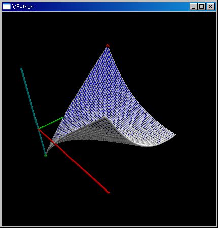
plot3dGr(..) は二次元平面上に分布する関数を 3D 表示します。
#(x^2-3xy+y^2)/(3+x+y) のニ変数有理関数のグラフを三次元表示させる
# 表示領域は x ∈ [-1,1], y ∈ [-1,1] の正方形領域
plot3dGr((`X^2- 3`X `Y + `Y^2)/(3+`X+`Y), [-1,1])
#
# 表示領域は 実数∈ [-2,2], 虚数∈ [-2i,2i] の領域
plot3dGr((`X^2+`X+1)/(`X^2-1), [-2,2],[-2 `i, 2 `i])
plot3dGr(sqrt(1-`X^2-`Y^2),[-0.5, 0.5])
plot3dGr(sqrt(1-`X^2-`Y^2),[-1,1])
vsGraph.py について
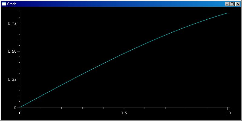
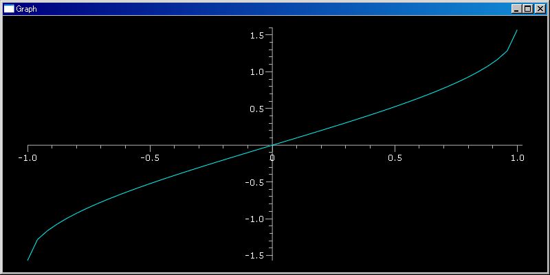
plotGr(arctan, -3,3)
plotGr([arctan(x) for x in klsp(-3,3)])
plotGr(arctan, klsp(-3,3))

plotGr(arctan( klsp(-3,3)))
<== plotGr(arctan( klsp(-3,3))) はufunc である必要がある
    <== arctan( klsp(-3,3)) がベクトルを返す関数であることを前提としているから
        <== 1 引数だけだから
plotGr(arctan, -3,3);plotGr(cos, -2,1, color=red)
注意
plotGr(arctan, [-3,3]) の書き方をしないでください。
plotGr([arctan(-3),arctan(3)]) の意味になります。二点を結んだ直線になります。
plotGr(arctan, -3,3) の書き方をする必要があります。
数学で関数の定義域を [-3,3] と表すことが多いので、誤って書いてしまうことがあります。
<== python では [...] はリストをあらわします。
<== plotGr([...]) はリストをグラフ化します。
plotgr(λ ω:exp(`i ω), -pi, pi)
plotTmCh
help(plotTmCh)
plotTmCh(vctMtrxAg)
    ' plot time chart for vector,array or matrix dictionary data
    '
example
グラフ表示のカスタマイズ
sc.source(plotGr)

def plotGr(vctAg, start=(), end=None, N=50, color = sf.cyan):
    """' plot graph for a function or vector data
        If you call plotGr(..) a number of times, then the graphs were plotted
        in piles.

        start,end are domain parameters, which are used if vctAg type is
        function

        if you want to vanish the graph then do as below
            objAt=plotGr(..)
                .
                .
            objAt.visible = None

    usage:
        plotGr(sin) # plot sin graph in a range from 0 to 1

        plotGr(sin,-3,3) #plot sin in a range from -3 to 3

        plotGr(sin,[-3,-2,0,1])
        # plot sequential line graph by
        #                       [(-3,sin(-3),(-2,sin(-2),(0,sin(0),(1,sin(1)]

        plotGr([sin(x) for x in klsp(-3,3)]) # plot a sequence data
    '"""

    vs = sf.vr()

    global __objGrDisplayGeneratedStt
    color = tuple(color)   # color argment may be list/vector
    import visual.graph as vg
    if __objGrDisplayGeneratedStt == None:
        __objGrDisplayGeneratedStt = vg.gdisplay()
    grphAt = vg.gcurve( color = color)
    #grphAt = vg.gcurve(gdisplay=dspAt, color = color)
    #import pdb; pdb.set_trace()
    if '__call__' in dir(vctAg):
        # vctAg is function
        if start != () and end == None and hasattr(start, '__iter__'):
            for x in start:
                grphAt.plot(pos = [x, float(vctAg(x))] )
        else:
            if start == ():
                start = 0
            if end == None:
                end = 1

            assert start != end
            if start > end:
                start, end = end, start

            #assert start != end
            """'
            for x in arsq(start, N, float(end-start)/N):
                # 08.10.27 add float(..) cast to avoid below error
                # "No registered converter was able to produce a C++ rvalue"
                # at ;;n=64;plotGr([sf.sc.comb(n,i) for i in range(n)])
                grphAt.plot(pos = [x, float(vctAg(x))] )
            '"""
            for x in sf.klsp(start, end, N):
                # 09.12.03 to display end and avoid 0
                grphAt.plot(pos = [x, float(vctAg(x))] )

        #return grphAt
        return __objGrDisplayGeneratedStt
    else:
        if (start != ()) or (end != None):
            #import pdb; pdb.set_trace()
            if start == ():
                start = 0
            if end == None:
                end = 1

            assert start != end
            if start > end:
                start, end = end, start

            N = len(vctAg)
            for i, x in enmasq([start, N, (end - start)/N]):
                grphAt.plot(pos = [x, float(vctAg[i])] )
        else:
            for i in range(len(vctAg)):
                grphAt.plot(pos = [i, float(vctAg[i])] )
        #return grphAt
        return __objGrDisplayGeneratedStt
 plotGr(sin5)
plotGr(vctAg, start=(), end=None, N=50, color=(0, 1, 1))
help(plotGr)
klsp
plotGr
一引数関数のグラフ表示
定義域 lower, upper
klsp
シーケンス・データの表示
renderMtrx(..)
二重表示
plotTmCh
plotTrajectory
renderMtCplxWithRGB
help(vsGraph)
N=32;plotGr(abs(fft(range(N))))
plotGr(sin5)
plotGr(vctAg, start=(), end=None, N=50, color=(0, 1, 1))
help(plotGr)
klsp
plotGr
一引数関数のグラフ表示
定義域 lower, upper
klsp
シーケンス・データの表示
renderMtrx(..)
二重表示
plotTmCh
plotTrajectory
renderMtCplxWithRGB
help(vsGraph)
N=32;plotGr(abs(fft(range(N))))
help(kNumeric)
■ 応用例
sqrt(1-`X^2-`Y^2) と接平面
Mathematica 例題
∂J(sqrt(1-`X^2-`Y^2),inDim=2)(0.4, 0.4)
===============================
[-0.48507125 -0.48507125]
---- ClTensor ----

[1,0,-0.48507125] と [0,1,-0.48507125] が接平面の傾きに沿ったベクトル
<== [0.4, 0.4, sqrt(...)(0.4, 0.4)] のオフセット位置で接平面を描く行列データを作成する
■■ Basic Functions
ClAF
    f,g=ClAF(sin), ClAF(cos);  f(2 f g + 3 g)(pi/3)
    ===============================
    0.700121217943
    f, g =ClAFM(sc.arctan2),ClAFM(λ x,y:[2x+y,x+2y]); f(g)(5,6)
    ===============================
    0.755104403479
f=λ x:2x;(sin + f)(1)
===============================
2.84147098481
(sin + (λ x:2x))(1)
===============================
2.84147098481
(sin + λ x:2x )(1)
invalid syntax (
ClAF 一変数関数の組み合わせによる多変数関数の合成
<
┌────────┐ ┌────────┐ ┌─────────┐
│┌──────┐│・・・│┌──────┐│ │┌──────┐ ┌──┬──┬──・──┐
││exp, sin, ││・←・││exp, sin, ││←││exp, sin, │←─┤0th │1st │2nd ・last│
││cos, tan, ││・関・││cos, tan, ││関││cos, tan, │ └┬─┴┬─┴┬─・┬─┘
││sinh, cosh, ││・←・││sinh, cosh, ││←││sinh, cosh, │`X ←┘ │ │ │
││tanh, arcsin││・数・││tanh, arcsin││数││tanh, arcsin│`Y ←───┘ │ │
││arccos, ││・←・││arccos, ││←││arccos, │`Z ←──────┘ │
││arctan, log,││・合・││arctan, log,││合││arctan, log,│`T ←─────────┘
││log10, sqrt ││・←・││log10, sqrt ││←││log10, sqrt │ the last element
│└──────┘│。成。│└──────┘│成│└──────┘` │
│ │ ← │ │←│ │
│ 加減乗除べき乗│ │ 加減乗除べき乗│ │ 加減乗除べき乗 │
│ よる混ぜ合わせ│ │ よる混ぜ合わせ│ │ よる混ぜ合わせ │
└────────┘ └────────┘ └─────────┘
例 ・・・ 3 cos(`Z) `Z
・・・ tan(2 sin +`X) 2 sin + `X
sin( .. exp(-X^2)..)・・・ exp(-X^2) `X^2
sy();span=~[-2,2];erf=ClAF(ss.erf);plot3dGr(erf sin, span, `i span)
putPv
putPv(~[[16,3,2,13],[5,10,11,8],[9,6,7,12],[4,15,14,1]], "magic")

Python sf プリプロセッサは 「:=」によるアサインでも putPv(..) の機能を行わせます
magic:=~[[16,3,2,13],[5,10,11,8],[9,6,7,12],[4,15,14,1]]
===============================
[[ 16.   3.   2.  13.]
 [  5.  10.  11.   8.]
 [  9.   6.   7.  12.]
 [  4.  15.  14.   1.]]
---- ClTensor ----
type magic.pvl

# python object printed out by pprint
ClTensor([[ 16.,   3.,   2.,  13.],
       [  5.,  10.,  11.,   8.],
       [  9.,   6.,   7.,  12.],
       [  4.,  15.,  14.,   1.]])
getPv
magic = sf.getPv('magic')
下のように読み出したほうが python sf らしいでしょう。
=:magic; 2 magic
===============================
[[ 32.   6.   4.  26.]
 [ 10.  20.  22.  16.]
 [ 18.  12.  14.  24.]
 [  8.  30.  28.   2.]]
---- ClTensor ----
shftSq,rttSq
shftSq(range(2,10))
===============================
[0, 2, 3, 4, 5, 6, 7, 8]

shftSq(range(2,10),3)
===============================
[0, 0, 0, 2, 3, 4, 5, 6]

shftSq(range(2,10),-3)
===============================
[5, 6, 7, 8, 9, 0, 0, 0]

shftSq(tuple(range(1,10)))
===============================
(0, 1, 2, 3, 4, 5, 6, 7, 8)

shftSq(~[range(1,10)])
[ 0.  1.  2.  3.  4.  5.  6.  7.  8.]
---- ClTensor ----
shftSq(~[range(1,10)])
[ 0.  1.  2.  3.  4.  5.  6.  7.  8.]
---- ClTensor ----

shftSq(~[range(1,10)].reshape(3,3))
===============================
[[ 0.  0.  0.]
 [ 1.  2.  3.]
 [ 4.  5.  6.]]
---- ClTensor ----

shftSq(sc.arange(1,10).reshape(3,3))
===============================
[[0 0 0]
 [1 2 3]
 [4 5 6]]
rttSq(range(2,10))
===============================
[9, 2, 3, 4, 5, 6, 7, 8]

rttSq(range(2,10),3)
===============================
[7, 8, 9, 2, 3, 4, 5, 6]

rttSq(range(2,10),-3)
===============================
[5, 6, 7, 8, 9, 2, 3, 4]

shftSq(tuple(range(1,10)))
===============================
(0, 1, 2, 3, 4, 5, 6, 7, 8)

shftSq(~[range(1,10)])
[ 0.  1.  2.  3.  4.  5.  6.  7.  8.]
---- ClTensor ----
rttSq(~[range(1,10)])
===============================
[ 9.  1.  2.  3.  4.  5.  6.  7.  8.]
---- ClTensor ----

rttSq(~[range(1,10)].reshape(3,3))
===============================
[[ 7.  8.  9.]
 [ 1.  2.  3.]
 [ 4.  5.  6.]]
---- ClTensor ----

rttSq(sc.arange(1,10).reshape(3,3))
===============================
[[7 8 9]
 [1 2 3]
 [4 5 6]]
product
product はシーケンス・データの要素を足し合わせたものを返します。sum(..) の + の代わりに * にした働きをします。
invF
sc.source(invF)
In file: D:\my\vc7\mtCm\pysf\basicFnctns.py
def invF(f, rangeLeft=-1,rangeRight=1):
"""' Return inversed function. Default range of value is [-1,1]
Cation! For inv(f)(x),
the sign(f(x)-rangeLeft) * sign(f(x)-rangeRight) must be -1
e.g.
invF(sin)(pi/6)
===============================
0.551069583099
invF(sin,-pi/2, pi/2)(0.1)
===============================
0.100167421161
'"""
return lambda x:sf.so_().brentq(lambda t:f(t)-x, rangeLeft, rangeRight)
===============================
None
combinate
list(combinate(list('abcd'),3))
===============================
[('a', 'b', 'c'), ('a', 'b', 'd'), ('a', 'c', 'd'), ('b', 'c', 'd')]
list(combinate([0,1,2,3],2))
===============================
[(0, 1), (0, 2), (0, 3), (1, 2), (1, 3), (2, 3)]
permutate
tuple(sf.permutate([2,1,0]))
===============================
(((2, 1, 0), 1), ((2, 0, 1), -1), ((1, 2, 0), -1), ((1, 0, 2), 1)
, ((0, 2, 1), 1), ((0, 1, 2), -1))
tuple(sf.permutate([0,1,2]))
===============================
(((0, 1, 2), 1), ((0, 2, 1), -1), ((1, 0, 2), -1), ((1, 2, 0), 1)
, ((2, 0, 1), 1), ((2, 1, 0), -1))
sc.source(`Λ)
def k__bq__lLambda____(*tplVctAg):
"""' return Wedge product tensor for vectors
'"""
def getTensor(tplIndex, *tplVctAg):
kryAt = sf.krry(tplVctAg[tplIndex[0]])
for i in range(1, len(tplIndex)):
kryAt = kryAt ^ sf.krry(tplVctAg[tplIndex[i]])
return kryAt
n = len(tplVctAg)
# confirm that all elements in tplVctAg are same length vector
lenAt = len(tplVctAg[0])
for k in range(n):
assert lenAt == len(tplVctAg[k])
krryAt = sf.kzrs(*([len(tplVctAg[0])]*n))
for index, sign in sf.permutate(range(n)):
krryAt = krryAt + sign * getTensor(index, *tplVctAg)
return krryAt
===============================
None
`Λ([1,2,3], [4,5,6])
===============================
[[ 0. -3. -6.]
[ 3. 0. -3.]
[ 6. 3. 0.]]
---- ClTensor ----
`Λ([1,2,3], [4,5,6], [7,8,0])
===============================
[[[ 0. 0. 0.]
[ 0. 0. 27.]
[ 0. -27. 0.]]
[[ 0. 0. -27.]
[ 0. 0. 0.]
[ 27. 0. 0.]]
[[ 0. 27. 0.]
[-27. 0. 0.]
[ 0. 0. 0.]]]
---- ClTensor ----
`Λ(`σx, `σy)
===============================
[[[[ 0.+0.j 0.+0.j]
[ 0.+0.j 0.+0.j]]
[[ 0.+0.j 0.+0.j]
[ 0.+2.j 0.+0.j]]]
[[[ 0.+0.j 0.-2.j]
[ 0.+0.j 0.+0.j]]
[[ 0.+0.j 0.+0.j]
[ 0.+0.j 0.+0.j]]]]
---- ClTensor ----
compose
compose(sin, cos)(0)
===============================
0.841470984808
compose(λ x:x^2, λ x:x*2)(3.0)
===============================
36.0
others
compose(f,g)
compose(sin, cos)(0)
===============================
0.841470984808
compose(λ x:x^2, λ x:x*2)(3)
===============================
36
bin(..)
bin_(..)
bin_(16)
===============================
0b1_0000
bin_(16, 32) # 32bit length
===============================
0b0000_0000__0000_0000___0000_0000__0001_0000
bin_(16.125)
===============================
0b1_0000
bin_(256+33, 5) # not five digit
===============================
0b1__0010_0001
pp(..)
pp(~[3.5, 4.0, 7.1])
[ 3.5, 4, 7.1]
-------- pp --
===============================
None
`σy
===============================
[[ 0.+0.j 0.-1.j]
[ 0.+1.j 0.+0.j]]
---- ClTensor ----
pp(`σy)
[[ 0, -1j]
,[ 1j, 0]]
-------- pp --
===============================
invF
sciIntf.py
invF(arctan)(0.5)
===============================
0.546302489844
invF(arctan)(1.1)
f(a) and f(b) must have different signs at excecuting:invF(arctan)(1.1)
■■ kNumeric scipy インターフェース
微分
積分
qdrt:積分
b
qdrt(f, a, b) ≡ ∫ f(x) dx
a
qdrt(sin,0,pi)
===============================
2.0
qdrt(sin, pi, 0)
===============================
-2.0
qdrt(λ x:exp(-x^2), -sc.inf, sc.inf)
===============================
1.77245385091
+∞
∫ exp(-x^2) dx
-∞
√π;; sqrt(pi)
===============================
1.77245385091
qdrt(λ x:exp(-x^2), sc.inf, -sc.inf)
(33, 'Domain error') at excecuting:qdrt(lambda x:exp(-x**2), sc.inf, -sc.inf)
si.quad(sin, 0,pi)
===============================
(2.0, 2.2204460492503131e-014)
quadAn:解析関数の線積分
quadAn(λ z:1/z, [1+`i,1-`i, -1-`i,-1+`i,1+`i])
===============================
(-6.2831853071795871j, 3.0615980059724259e-014, 6.9757369942584612e-014)
quadAn(λ z: z**2, [1+`i,1-`i, -1-`i,-1+`i,1+`i])
===============================
(0j, 7.3849307489406795e-014, 7.3849307489406795e-014)
quadAn(λ z:1/z**2, [1+`i,1-`i, -1-`i,-1+`i,1+`i])
===============================
(0j, 5.0593736107878128e-014, 5.0593736107878128e-014)
quadAn(log, [1+`i,1-`i, -1-`i,1-`i,1+`i])
===============================
(-2.2204460492503131e-016j, 3.238252998456195e-009, 3.2383033509434062e-009)
quadN:多次元空間での線積分
vctE = λ vctP:vctP/norm(vctP);quadN(vctE, ([1,1,1],[1,2,3]) )
===============================
(2.0096065792050641, 2.2311114946716608e-014)
vctE = λ vctP:vctP/norm(vctP);quadN(vctE, ([1,1,0],[1,-1,0],[-1,-1,0],[-1,1,0],[1,1,0]) )
===============================
(2.8130846960094083e-017, 3.6623805685846749e-014)
quadGN:多次元空間ての Gauss 積分法を使った線積分
vctE = λ vctP:vctP/norm(vctP);quadGN(vctE, ([1,1,1],[1,2,3]) )
===============================
(2.0096065781679306, 7.8044882778627311e-009)
vctE = λ vctP:vctP/norm(vctP);quadGN(vctE, ([1,1,0],[1,-1,0],[-1,-1,0],[-1,1,0],[1,1,0]) )
===============================
(0.0, 0.0)
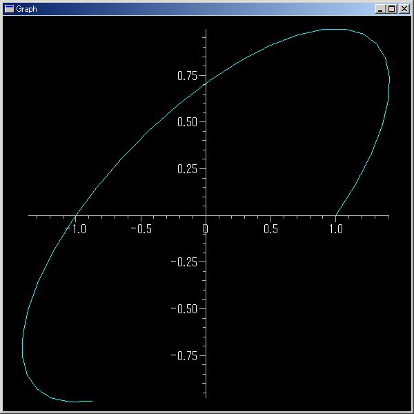
cOdeInt:複素数値微分方程式の積分
//@@
# 10.02.06 Harmonic Oscilator by step
import pysf.sfFnctns as sf
def func(psi, x):
return 1/1j * psi
N = 30
#y = sf.cOdeInt( func, [1+1j, 0], sf.arSqnc(0,N,5.0/N) )
y = sf.cOdeInt( func, [1+1j], sf.arSqnc(0,N,5.0/N) )
print y
sf.plotTrajectory([(x.real, x.imag) for x in y[:,0]])
//@@@
//copy c:\#####.### temp.py /y
//temp.py
[[ 1.00000000+1.j ]
[ 1.15203938+0.82024708j]
[ 1.27215166+0.61776221j]
[ 1.35700810+0.39815699j]
[ 1.40425705+0.16751743j]
[ 1.41258907-0.06776463j]
[ 1.38177327-0.30116869j]
[ 1.31266364-0.5262263j ]
[ 1.20717546-0.73670032j]
[ 1.06823217-0.92675777j]
[ 0.89968440-1.09113149j]
[ 0.70620319-1.22526609j]
[ 0.49315060-1.32544424j]
[ 0.26643106-1.38888964j]
[ 0.03232778-1.41384399j]
[-0.20267144-1.39961575j]
[-0.43205391-1.34659919j]
[-0.64946264-1.25626361j]
[-0.84887247-1.13111252j]
[-1.02475703-0.9746143j ]
[-1.17224196-0.79110607j]
[-1.28723991-0.58567349j]
[-1.36656389-0.36400983j]
[-1.40801556-0.13225816j]
[-1.41044613+0.10315884j]
[-1.37378825+0.33571695j]
[-1.29905785+0.55897116j]
[-1.18832595+0.7667343j ]
[-1.04466134+0.95324852j]
[-0.87204547+1.11334484j]]
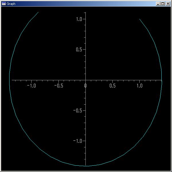
二次元調和振動子
初期位置 (1,0)
初期速度 (1,1): (1j,1j) での運動
X' =ΔX/(Δ(`i t))= ∂H(Z)/∂P == -`i Z.imag
P' =ΔP/(Δ(`i t))= ∂H(Z)/∂X == Z.real
H(p,x) = 1/2(x^2+p^2) == H(P,X) == 1/2(X^2 - P^2) where X∈real, P∈imaginaryNumber
//@@
# 10.02.06 Harmonic Oscilator by step
import pysf.sfFnctns as sf
def func(psi, x):
return 1/1j * psi
N = 30
#y = sf.cOdeInt( func, [1+1j, 0], sf.arSqnc(0,N,5.0/N) )
y = sf.cOdeInt( func, [1+1j, 1j], sf.arSqnc(0,N,5.0/N) )
print y[:,0]
sf.plotTrajectory([(x[0].real, x[1].real) for x in y])
//@@@
//copy c:\#####.### temp.py /y
//temp.py
//@@
import pysf.sfFnctns as sf
N=100
N=10
def func(x,t):
print "Now in func. x=",x, " t=",t
return 1
y = sf.si.odeint( func, 1, sf.arSqnc(0,N,5.0/N) )
print y
sf.plotGr(y)
//@@@
//copy c:\#####.### temp.py /y
//temp.py
Now in func. x= [ 1.] t= 0.0
Now in func. x= [ 1.00005921] t= 5.92128761832e-005
Now in func. x= [ 1.00011843] t= 0.000118425752366
Now in func. x= [ 1.59224719] t= 0.592247187584
Now in func. x= [ 2.18437595] t= 1.18437594942
Now in func. x= [ 2.77650471] t= 1.77650471125
Now in func. x= [ 8.69779233] t= 7.69779232956
[[ 1. ]
[ 1.5]
[ 2. ]
[ 2.5]
[ 3. ]
[ 3.5]
[ 4. ]
[ 4.5]
[ 5. ]
[ 5.5]]
■ nearlyEq:near 判定
sc.source(nearlyEq)
In file: D:\my\vc7\mtCm\pysf\kNumeric.py
def nearlyEq(lftAg, rhtAg, tolerance=1e-6):
"""' compare with small tolerance to test float/complex values which may
contain a tolerance. In many cases, if the first 6 digits of two terms
are same, then we can see them as same. In that cases, nearlyEq(..)
function is usefull.
Subtrac:'lftAg - rhtAg' must have a value
If lftAg is tuple or list or dict, we convert it to a ClTensor instance and
enabel to subtract.
usage:
nearlyEq(3, 3.0000000001) # return True
nearlyEq(3, 3.01) # return False
nearlyEq(~[3,4], [3.0000000001, 4]) # return True
nearlyEq( [3,4], [3.0000000001, 4]) # return True
nearlyEq( [3,4], [3.01 , 4]) # return False
nearlyEq([3,3.00000001], 3) # True, ~[,3.00000001] - 3 has a value
'"""
if isinstance(lftAg,(tuple,list,dict)):
lftAg = sf.ClTensor(lftAg)
return norm(lftAg-rhtAg) <= max(norm(lftAg), norm(rhtAg))*tolerance
===============================
None
偏微分方程式
┌──────┐ +--------+
│境界条件行列│ | 漸化式 |
└───┬──┘ +---------
↓ ↓
+--------------------------+
| soveLaplacian(..) |
| or solvePDE(.. ) |
| or itrSlvPDE(..) |
+--------------------------+
↓
dctRslt:数値解行列
↓
renderMtrx(dctRslt):数値解の可視化
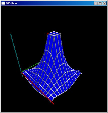
境界条件行列
solveLaplacian
N=14;mt=kzrs(N,N,object);mt.fill(True);mt[6:9,6:9]=[[1,1,1]]*3;mtBndry:=mt
===============================
[[True True True True True True True True True True True True True True]
[True True True True True True True True True True True True True True]
[True True True True True True True True True True True True True True]
[True True True True True True True True True True True True True True]
[True True True True True True True True True True True True True True]
[True True True True True True True True True True True True True True]
[True True True True True True 1 1 1 True True True True True]
[True True True True True True 1 1 1 True True True True True]
[True True True True True True 1 1 1 True True True True True]
[True True True True True True True True True True True True True True]
[True True True True True True True True True True True True True True]
[True True True True True True True True True True True True True True]
[True True True True True True True True True True True True True True]
[True True True True True True True True True True True True True True]]
---- ClTensor ----
=:mtBndry;renderMtrx(solveLaplacian(mtBndry))
index:(6, 6) max: 1
index:(7, 13) min:-0.174644
===============================
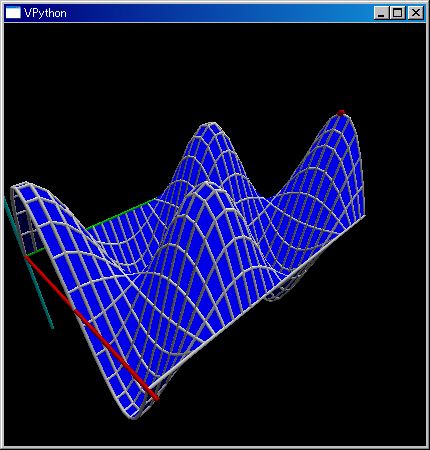
solvePDE
N,M=30,20;mt=kzrs(M,N,object);mt.fill(True);mt[:,0],mt[:,1]=[sin(klsp(0,2pi,M))]*2;mt[0,:],mt[M-1,:]=[[0]*N]*2;mtBndry:=mt
===============================
[[0 0 0 0 0 0 0 0 0 0 0 0 0 0 0 0 0 0 0 0 0 0 0 0 0 0 0 0 0 0]
[0.324699469205 0.324699469205 True True True True True True True True
True True True True True True True True True True True True True True
True True True True True True]
[0.61421271269 0.61421271269 True True True True True True True True True
True True True True True True True True True True True True True True
True True True True True]
[0.837166478263 0.837166478263 True True True True True True True True
True True True True True True True True True True True True True True
True True True True True True]
[0.969400265939 0.969400265939 True True True True True True True True
True True True True True True True True True True True True True True
True True True True True True]
[0.996584493007 0.996584493007 True True True True True True True True
True True True True True True True True True True True True True True
True True True True True True]
[0.915773326655 0.915773326655 True True True True True True True True
True True True True True True True True True True True True True True
True True True True True True]
[0.735723910673 0.735723910673 True True True True True True True True
True True True True True True True True True True True True True True
True True True True True True]
[0.475947393037 0.475947393037 True True True True True True True True
True True True True True True True True True True True True True True
True True True True True True]
[0.164594590281 0.164594590281 True True True True True True True True
True True True True True True True True True True True True True True
True True True True True True]
[-0.164594590281 -0.164594590281 True True True True True True True True
True True True True True True True True True True True True True True
True True True True True True]
[-0.475947393037 -0.475947393037 True True True True True True True True
True True True True True True True True True True True True True True
True True True True True True]
[-0.735723910673 -0.735723910673 True True True True True True True True
True True True True True True True True True True True True True True
True True True True True True]
[-0.915773326655 -0.915773326655 True True True True True True True True
True True True True True True True True True True True True True True
True True True True True True]
[-0.996584493007 -0.996584493007 True True True True True True True True
True True True True True True True True True True True True True True
True True True True True True]
[-0.969400265939 -0.969400265939 True True True True True True True True
True True True True True True True True True True True True True True
True True True True True True]
[-0.837166478263 -0.837166478263 True True True True True True True True
True True True True True True True True True True True True True True
True True True True True True]
[-0.61421271269 -0.61421271269 True True True True True True True True
True True True True True True True True True True True True True True
True True True True True True]
[-0.324699469205 -0.324699469205 True True True True True True True True
True True True True True True True True True True True True True True
True True True True True True]
[0 0 0 0 0 0 0 0 0 0 0 0 0 0 0 0 0 0 0 0 0 0 0 0 0 0 0 0 0 0]]
---- ClTensor ----
=:mtBndry;N,M,timeWidth=30,20,1.5;mt=kzrs(M,N);mt.fill(0);def f(mt,(j,k)): mt[j,k]=2mt[j,k-1]-mt[j,k-2]+(timeWidth*M/N)^2 (mt[j+1,k-1]+mt[j-1,k-1]-2mt[j,k-1]);renderMtrx(solvePDE(mtBndry,f,40))
N,M=30,20;mt=kzrs(M,N,object);mt.fill(True);mt[0,:]=[0]*N;mt[0,0:10]=sin(klsp(0,2pi,10));mt[:,0]=[0]*M;mt[:,1]=[0]*M;mtBndry:=mt
=:mtBndry;N,M,timeWidth=30,20,1.5;mt=kzrs(M,N);mt.fill(0);def f(mt,(j,k)): mt[j,k]=2mt[j,k-1]-mt[j,k-2]+(timeWidth*M/N)^2 (mt[j+1,k-1]+mt[j-1,k-1]-2mt[j,k-1]);renderMtrx(solvePDE(mtBndry,f,40))
itrSlvPDE
=:mtBndry;N,M,timeWidth=30,20,1.5;mt=kzrs(M,N);mt.fill(0);for mt,(j,k) in itrSlvPDE(mtBndry,40):mt[j,k]=2mt[j,k-1]-mt[j,k-2]+(timeWidth*M/N)^2 (mt[j+1,k-1]+mt[j-1,k-1]-2mt[j,k-1]);renderMtrx(mt)
dct2(sq)
dct2([0.7, 0.6, 0.95, 0.85, 0.55, 0.1, 0.68, 0.43])
===============================
[ 1.71826948 0.36452813 -0.08071514 -0.38011727 0.07071068 0.32186722
-0.15790841 0.2548168 ]
---- ClTensor ----
dct2(range(32))
===============================
[ 8.76812409e+01 -5.18555951e+01 -2.04281037e-14 -5.74305749e+00
-5.32907052e-15 -2.05378057e+00 0.00000000e+00 -1.03699056e+00
-1.15463195e-14 -6.18143249e-01 8.88178420e-16 -4.05658019e-01
2.13162821e-14 -2.82932996e-01 -9.76996262e-15 -2.05367296e-01
8.43769499e-14 -1.52902657e-01 3.64153152e-14 -1.15420131e-01
1.42108547e-14 -8.73494434e-02 -4.39648318e-14 -6.53996651e-02
1.02140518e-14 -4.75025193e-02 -3.28626015e-14 -3.22782075e-02
-6.43929354e-15 -1.87448835e-02 -8.65973959e-15 -6.14826207e-03]
---- ClTensor ----
■■ rational 数値式の有理多項式とインパルス・インディシャル応答
`X は有理式の X を ClAF 化したものとする。
<== べき乗 ClAF と ClRational の両立は、混乱のもと
<== ClRational の list 値が
(3+`s^2+`s)(range(5))
===============================
[ 3. 5. 9. 15. 23.]
k__bq_X___ = sf.ClAF(k__bq_s___) # `X
で作った `X を `s の代わりにできない
<== `X の scalar 係数の掛け算と加減乗除算で 有理式を表現できる。でも ClAF のインスタンスになってしまう。ClRational のインスタンスではない。だから ClRational に属するメソッドを呼び出せない。
plotBode( (`s+1)/(`s^2+`s+1), 0.01 )
OK
( (`X+1)/(`X^2+`X+1), 0.01 ).getAnRspns(..)
plotBode( (`X+1)/(`X^2+`X+1), 0.01 )
Traceback (most recent call last):
File "sfPP.py", line 2, in
R1,R2,L,C=1Ω`,1kΩ`,10uH`,1uF`; Z1,Z2 =L `s + R1, R2 ~+ (1/(C `s));(Z2/(Z1+Z2)).plotBode(1Hz`, 1 M` Hz`)
R1,R2,L,C=1Ω`,1kΩ`,10uH`,1uF`; Z1,Z2 =L `s + R1, R2 ~+ (1/(C `s)); Z2/(Z1+Z2).plotBode(1Hz`, 1 M` Hz`)
注意2
■■ tlRcGn 再帰・繰り返し
■ 無限数列
mkSrs(..): 関数引数から無限数列の生成
N=5;tn.mkSrs( λ n:0.75^n sin(n pi/6) )[:N]
===============================
[0.0, 0.37499999999999994, 0.4871392896287467, 0.421875, 0.27401585041617005]
■■ vsGraph
vs();vs.sphere(pos=[1,2,3], radius=1,color=red);vs.box(pos=[0,0,0], axis=[0.5,1,1], height = 1, width = 0.5)
//@@
from __future__ import division
# -*- encoding: cp932 -*-
from pysf.sfFnctns import *
setDctGlobals(globals())
from pysf.customize import *
if os.path.exists('.\sfCrrntIni.py'):
from sfCrrntIni import *
print sy_
print sy
sy()
print sy_
print sy
//@@@
■■ rational ClRtnl
( (`s-1)/(`s+1) ).plotBode(0.001,100)
横軸の単位は周波数です。Radian/sec ではありません。
open loop;;=:Gs;Z1,Z2 = 1kΩ`,1/(10uF` `s);invF(-1 + Gs (Z2/(Z1+Z2)), 1e3,1e4)(0)
===============================
9930.0449999
←radian/sec
closed loop;;=:Gs;Z1,Z2 = 1kΩ`,1/( 1uF` `s);(1/(1/Gs +(Z2/(Z1+Z2)))).plotAnRspns(100ms`)
■■ oc: octn.py
■■ tn: tlRcGn.py
■■ symIntf
tu(), tt(),tr()
import sympy.physics.units as ut;1 * ut.A/(2 * ut.V)
===============================
A**2*s**3/(2*kg*m**2)
import sympy.physics.units as ut;1 * ut.A/(2 * ut.V)
tr();2.0A`/(3V`)
===============================
0.666666666666667*A`/V`
tr();2A`/(3V`)
===============================
2*A`/(3*V`)
tr();ts.cancel(2A`/(3V`))
■■ kmayavi
import enthought.mayavi.version as md;md.version
===============================
3.3.1
kmshw(..)
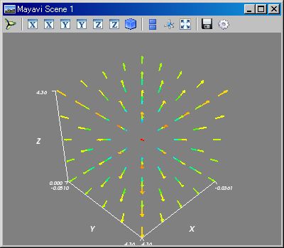
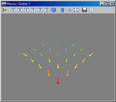
kqvr3d(..)
N=5;v=range(N);vcPs=[[[[x,y,z]for x in v]for y in v]for z in v] ;kqvr3d(vcPs,vcPs);kmshw()
N=5;v=range(N);vcPs=[[[[x,y,z]for x in v]for y in v]for z in v] ;kqvr3d(vcPs);kmshw()
N=5;v=range(N);vcPs=~[[[x,y] for x in v] for y in v] ;kqvr3d(vcPs);kmshw()
N=5;v=range(N);vcPs=~[[[x,y] for x in v] for y in v] ;kqvr3d(vcPs, vcPs);kmshw()
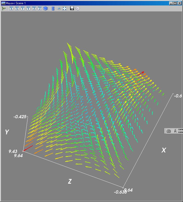
# 三次元対称行列によるベクトルの回転
v,mt=klsp(-1,1,10),~[[0,1,2],[1,0,1],[2,1,0]];val=[[[mt [z,y,x]for x in v]for y in v]for z in v];kqvr3d(val);kmshw()
三次元 I 行列 一引数;;v,mt=klsp(-1,1,6),~[[1,0,0],[0,1,0],[0,0,1]];val=[[[mt [z,y,x]for x in v]for y in v]for z in v];kqvr3d(val);kmshw()
三次元 I 行列 二引数;;v,mt=klsp(-1,1,6),~[[1,0,0],[0,1,0],[0,0,1]];val=[[[mt [z,y,x]for x in v]for y in v]for z in v];kqvr3d(val, val);kmshw()
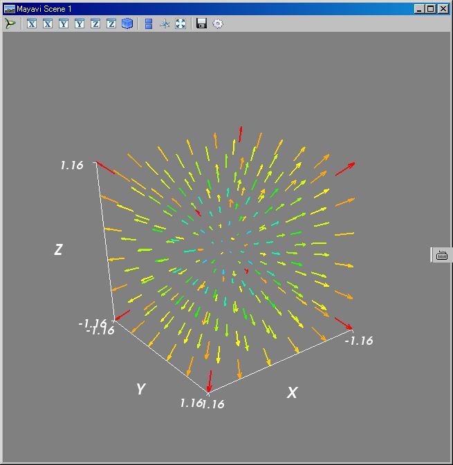
これが正しい x,y,z 方向;;N=10;v=range(N);vcPs=~[[[[z,y,x] for x in range(N)] for y in range(N)] for z in range(N)];kqvr3d(0.1 vcPs);mlb().axes();mlb().show()
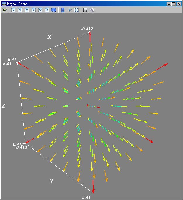
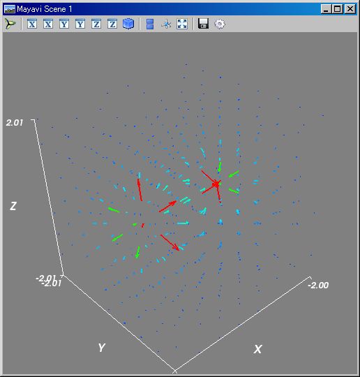
# dipole 電場分布
OK;;N=8;v=klsp(-2,2,N);f=λ r:(~[`X,`Y,`Z] - r)/normAF(~[`X,`Y,`Z] - r)^3;kqvr3d( (list(mrng(v,v,v))),f([1,0,0])-f([-1,0,0]) );kmshw()
■■ kre.py
/,% operator
kr=kre.krgl('^def\s*r');[str for str in open('pysf\vsGraph.py') if str/kr%0]
■■ cusomize.py
■ 微分
∂x
∂t
∂p,∂q は?
tr();∂x(`x)
tr();∂p(`p^2)
===============================
2*p
■■ モジュールごとの時間負荷
//@@
import time
startTimeAt = time.time()
import os
os.system("""python -m sfPP 3+4""")
print "Total executing time:",time.time() - startTimeAt
//@@@
Enthought 2.6 in MSI pysf0.95 customizeBig.py
protect 止め:ipconfit /all を実行しない
import tlRcGn as tn を customizeMiddle.py に追加
C:\my\vc7\mtCm>python temp.py
===============================
7
Total executing time: 2.59399986267
Total executing time: 1.60899996758
Total executing time: 1.60899996758
Total executing time: 1.60899996758
Total executing time: 1.60899996758
Total executing time: 1.625
Total executing time: 1.625
Total executing time: 1.60899996758
Total executing time: 1.60899996758
Total executing time: 1.60899996758
F:\my\vc7\mtCm>python temp.py
===============================
7
Total executing time: 3.61000013351
Total executing time: 2.5
Total executing time: 2.65600013733
Total executing time: 2.56299996376
Total executing time: 2.56299996376
Total executing time: 2.54700016975
Total executing time: 2.60899996758
Total executing time: 2.71900010109
Total executing time: 2.625
Total executing time: 2.54700016975
Enthought 2.6 in MSI pysf0.95 customizeMiddle
protect 止め:ipconfit /all を実行しない
import tlRcGn as tn を customizeMiddle.py に追加
C:\my\vc7\mtCm>python temp.py
===============================
7
Total executing time: 1.10899996758
Total executing time: 0.93799996376
Total executing time: 0.921999931335
Total executing time: 0.93700003624
Total executing time: 0.953999996185
Total executing time: 0.953000068665
Total executing time: 0.953000068665
Total executing time: 0.93700003624
Total executing time: 0.952999830246
Total executing time: 0.953000068665
F:\my\vc7\mtCm>python temp.py
===============================
7
Total executing time: 1.79699993134
Total executing time: 1.81200003624
Total executing time: 1.625
Total executing time: 1.54699993134
Total executing time: 1.51499986649
Total executing time: 1.5
Total executing time: 1.64100003242
Total executing time: 1.51600003242
Total executing time: 1.51600003242
Total executing time: 1.57800006866
Enthought 2.6 in MSI pysf0.95 customizeMiddle
protect 止め:ipconfit /all を実行しない
C:\my\vc7\mtCm>python temp.py
===============================
7
Total executing time: 1.07799983025
Total executing time: 0.968999862671
Total executing time: 0.93799996376
Total executing time: 0.93700003624
Total executing time: 0.93700003624
Total executing time: 0.952999830246
Total executing time: 0.93700003624
Total executing time: 0.93700003624
Total executing time: 0.922000169754
Total executing time: 0.93799996376
Total executing time: 0.93799996376
F:\my\vc7\mtCm>python temp.py
===============================
7
Total executing time: 3.26599979401
Total executing time: 1.51600003242
Total executing time: 1.57800006866
Total executing time: 1.54600000381
Total executing time: 1.56299996376
Total executing time: 1.67199993134
Total executing time: 1.51600003242
Total executing time: 1.53100013733
Total executing time: 1.48399996758
Total executing time: 1.54699993134
■■ kv:テスト
■■ ワンライナー構文 tips
ワンライナーでも if the else を行わせる
三項演算子 if else;;lst=[];for k in range(10):lst.append(k) if k>5 else None;lst
===============================
[6, 7, 8, 9]
■■ ワンライナー構文での Python の不具合
ループ変数を参照できない
for N in range(10):print (λ y:N y)(1)
global name 'N' is not defined at excecuting:for N in range(10):print (lambda y:N * y)(1)
//@@
print [ (lambda y:N*y)(1) for N in range(10)]
//@@@
[0, 1, 2, 3, 4, 5, 6, 7, 8, 9]
//@@
for N in range(10):
print (lambda y:N*y)(1)
//@@@
0
1
2
3
4
5
6
7
8
9
python -c "print 3+4"
7
python -c "for N in range(10):print (lambda y:N*y)(1)
invalid syntax (
poly1d 要素の行列を作れない
P=poly1d; ~[P([1,2,3]),P([4,5,6])]
===============================
[[3 2]
[6 5]]
---- ClFldTns:
//@@
import numpy as sc
P = sc.poly1d
print sc.array([P([1,2,3]),P([4,5,6])])
print
print sc.array([P([1,2,3]),P([4,5,6])],dtype=object)
//@@@
[[3 2]
[6 5]]
[[3 2]
[6 5]]
at Enthought 2.6
scalarStt
mailto: your@email.ne.jp
Last update: